pymead.core.bezier.Bezier#
- class Bezier(point_sequence: PointSequence, default_nt: int | None = None, name: str | None = None, t_start: float | None = None, t_end: float | None = None, **kwargs)[source]#
Bases:
ParametricCurve- __init__(point_sequence: PointSequence, default_nt: int | None = None, name: str | None = None, t_start: float | None = None, t_end: float | None = None, **kwargs)[source]#
Computes the Bézier curve through the control points \(\mathbf{P}_i\) according to
\[\mathbf{C}(t)=\sum_{i=0}^n \mathbf{P}_i B_{i,n}(t)\]where \(B_{i,n}(t)\) is the Bernstein polynomial, given by
\[B_{i,n}(t)={n \choose i} t^i (1-t)^{n-i}\]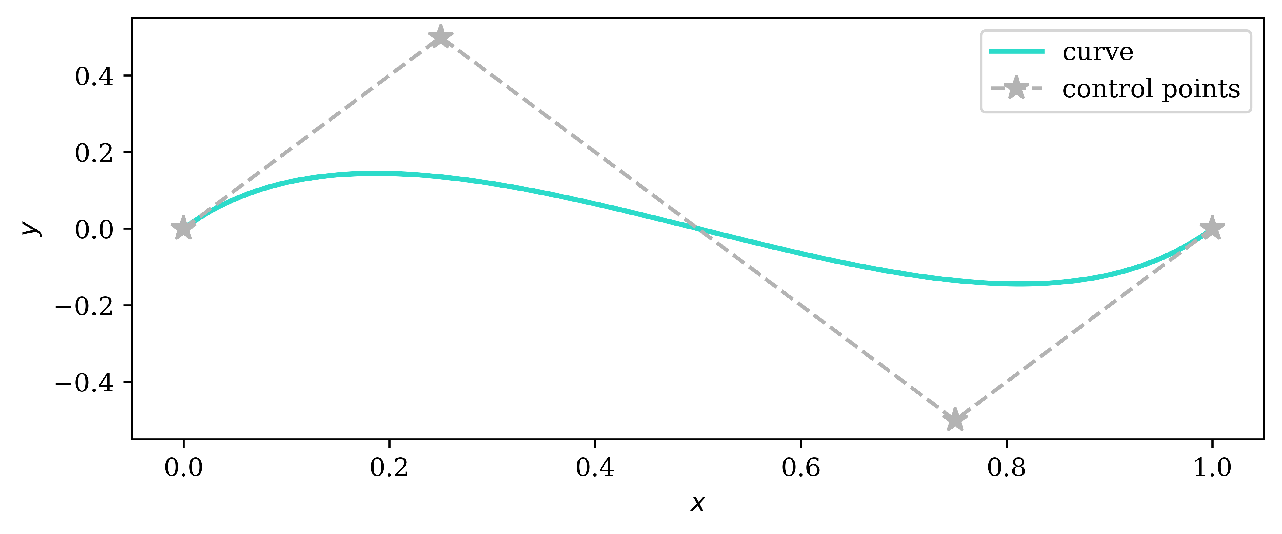
Cubic Bézier curve#
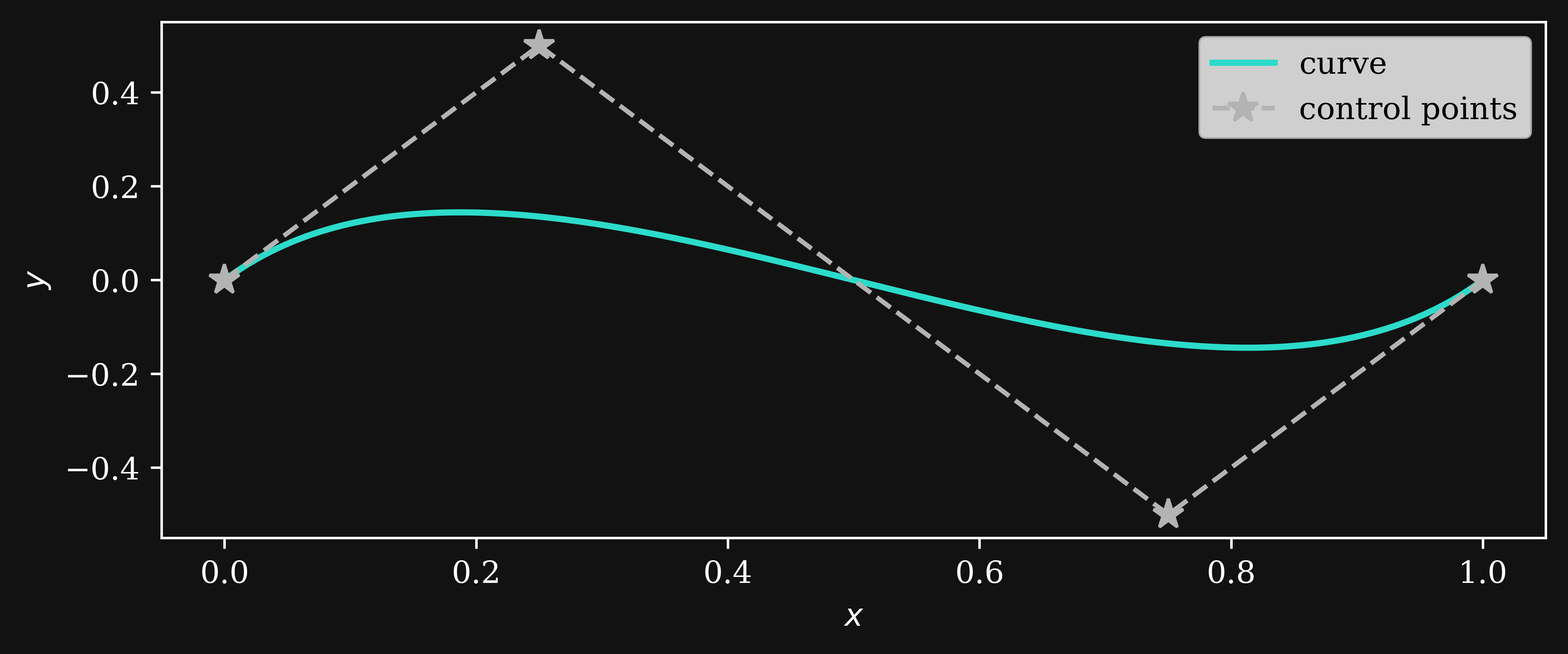
Cubic Bézier curve#
An example cubic Bézier curve (degree \(n=3\)) is shown above. Note that the curve passes through the first and last control points and has a local slope at \(P_0\) equal to the slope of the line passing through \(P_0\) and \(P_1\). Similarly, the local slope at \(P_3\) is equal to the slope of the line passing through \(P_2\) and \(P_3\). These properties of Bézier curves allow us to easily enforce \(G^0\) and \(G^1\) continuity at Bézier curve “joints” (common endpoints of connected Bézier curves).
- Parameters:
point_sequence (PointSequence) – Sequence of points defining the control points for the Bézier curve
name (str or
None) – Optional name for the curve. Default:Nonet_start (float or
None) – Optional starting parameter vector value for the Bézier curve. Not specifying this value automatically gives a value of0.0. Default:Nonet_end (float or
None) – Optional ending parameter vector value for the Bézier curve. Not specifying this value automatically gives a value of1.0. Default:None
Methods
bernstein_poly(n, i, t)Calculates the Bernstein polynomial for a given Bézier curve order, index, and parameter vector.
compute_t_corresponding_to_x(x_seek[, t0])compute_t_corresponding_to_y(y_seek[, t0])derivative(t, order)Calculates an arbitrary-order derivative of the Bézier curve.
evaluate([t])Evaluates the curve using an optionally specified parameter vector.
evaluate_xy([t])finite_diff_P(P, k, i)Calculates the finite difference of the control points as shown in https://pages.mtu.edu/~shene/COURSES/cs3621/NOTES/spline/Bezier/bezier-der.html
get_control_point_array()Gets a dictionary representation of the pymead object.
Generates another
Bezierobject representing the derivative ("hodograph") of the original curveinsert_point(idx, point)insert_point_after_point(point_to_add, ...)plot([ax, nt, show, save_file])Plots the airfoil to a
matplotlibfigure.point_removal_deletes_curve()point_sequence()points()remove()remove_point([idx, point])reverse_point_sequence()set_point_sequence(point_sequence)split(t_split)Attributes
- static bernstein_poly(n: int, i: int, t: int)[source]#
Calculates the Bernstein polynomial for a given Bézier curve order, index, and parameter vector. The Bernstein polynomial is described by
\[B_{i,n}(t)={n \choose i} t^i (1-t)^{n-i}\]- Parameters:
- Returns:
Array of values of the Bernstein polynomial evaluated for each point in the parameter vector
- Return type:
np.ndarray
- derivative(t: ndarray, order: int)[source]#
Calculates an arbitrary-order derivative of the Bézier curve.
- Parameters:
t (np.ndarray) – The parameter vector
order (int) – The derivative order. For example,
order=2returns the second derivative.
- Returns:
An array of
shape=(N,2)whereNis the number of evaluated points specified by the \(t\) vector. The columns represent \(C^{(m)}_x(t)\) and \(C^{(m)}_y(t)\), where \(m\) is the derivative order.- Return type:
np.ndarray
- evaluate(t: array | None = None, **kwargs) PCurveData[source]#
Evaluates the curve using an optionally specified parameter vector. Also included are first derivative, second derivative, and curvature information. These are given by
\[\mathbf{C}'(t)=n \sum_{i=0}^{n-1} (\mathbf{P}_{i+1} - \mathbf{P}_i) B_{i,n-1}(t)\]\[\mathbf{C}''(t)=n(n-1) \sum_{i=0}^{n-2} (\mathbf{P}_{i+2}-2\mathbf{P}_{i+1}+\mathbf{P}_i) B_{i,n-2}(t)\]\[\kappa(t)=\frac{C'_x(t) C''_y(t) - C'_y(t) C''_x(t)}{[(C'_x)^2(t) + (C'_y)^2(t)]^{3/2}}\]Here, the \('\) and \(''\) superscripts are the first and second derivatives with respect to \(x\) and \(y\), not the parameter \(t\). The result of \(\vec{C}''(t)\), for example, is a vector with two components, \(C''_x(t)\) and \(C''_y(t)\).
- Parameters:
t (np.ndarray or
None) – Optional direct specification of the parameter vector for the curve. Not specifying this value gives a linearly spaced parameter vector fromt_startort_endwith the default size. Default:Nonekwargs – Additional keyword arguments to pass to
ParametricCurve.generate_t_vec
- Returns:
Data class specifying the following information about the Bézier curve:
\[C_x(t), C_y(t), C'_x(t), C'_y(t), C''_x(t), C''_y(t), \kappa(t)\]where the \(x\) and \(y\) subscripts represent the \(x\) and \(y\) components of the vector-valued functions \(\mathbf{C}(t)\), \(\mathbf{C}'(t)\), and \(\mathbf{C}''(t)\).
- Return type:
- static finite_diff_P(P: ndarray, k: int, i: int)[source]#
Calculates the finite difference of the control points as shown in https://pages.mtu.edu/~shene/COURSES/cs3621/NOTES/spline/Bezier/bezier-der.html
- get_dict_rep()[source]#
Gets a dictionary representation of the pymead object. In general, this dictionary should consist of only the required arguments for object instantiation. For example, the dictionary representation of a point looks something like this:
{"x": 0.3, "y": 0.5}. If the argument requires a reference to aPymeadObjrather than a string or float value, thename()method should be the value that is stored. For an example, see the overridden value of this method inpymead.core.airfoil.Airfoil. All subclasses ofPymeadObjmust implement this method, since it is the way pymead objects are stored in saved instances of aGeometryCollection(.jmeafiles).
- hodograph() Bezier[source]#
Generates another
Bezierobject representing the derivative (“hodograph”) of the original curve- Returns:
Hodograph of the curve
- Return type:
- plot(ax: Axes | None = None, nt: int = 100, show: bool = True, save_file: str | None = None, **plt_kwargs)[source]#
Plots the airfoil to a
matplotlibfigure.- Parameters:
ax (plt.Axes or None) – Matplotlib Axes object on which the curve will be plotted. If specified, this method will only. If
None, a new figure will be created. Default:Nonent (int) – Number of parametric values to evaluate along the curve. Default: 100
show (bool) – Whether to immediately show the curve plot. Ignored if
axis notNone. Default:Truesave_file (str or None) – Name of the file to save. If
None, the curve image will not be saved to file. Ignored ifaxis notNone. Default:Noneplt_kwargs – Additional keyword arguments to pass to
matplotlib.pyplot.plot