Airfoil Matching

A common problem in airfoil design is matching an existing set of airfoil coordinates with a parametrization. For example, a design strategy might call for optimizing an airfoil using a NACA 0012 as a baseline airfoil. However, the NACA 0012 is defined by a simple polynomial function that might not be a useful parametrization scheme for more complex airfoil designs. Therefore, we can take an existing parametrization and find the set of design variables that makes the output airfoil most closely match the target NACA 0012 airfoil.

To start, we first add an Airfoil object to the canvas. See Geometric Objects for a guide on how to do this. Then, we need an airfoil coordinate file representing the target airfoil. This can be either the tag of an airfoil on Airfoil Tools or an airfoil coordinate file. The coordinate file must be in the Selig format, where the first point is the upper surface of the trailing edge, and the points move counter-clockwise to the lower surface of the trailing edge.

Note

The airfoil matching tool only works for a single airfoil at a time. To match multiple airfoils in a multi-element airfoil system to a set of target airfoils, each airfoil must be matched one at a time.

The matching process itself may be iterative to get the best results, using the following steps:

1. Generate a parametrization for the airfoil using points, lines, curves, and constraints, making sure to also generate an Airfoil object.

2. Promote any constraint values and point locations to design variables as needed.

3. Select a target airfoil and either obtain the tag of the airfoil from Airfoil Tools or create an airfoil coordinate file.

4. Match the airfoil.

5. If the match is not satisfactory, determine whether some or many of the design variables are at that bounds (use Ctrl+B to see/edit a table of the bounds values in the GUI). Expand the bounds of these variables as necessary. Additionally, it may be necessary to add or remove control points from the curves to get a better match.

6. Repeat steps 4 and 5 until an satisfactory solution is reached.

Important

To get the best results, make sure to align the trailing edge upper and lower surface points of the parametrized airfoil with those of the target airfoil.

A tutorial for matching the NACA 0012 using a built-in example in pymead is shown for both the API and GUI below.

GUI

To get a parametrization to start with, load in an airfoil pymead’s example directory by selecting File → Load Example → Shape Optimization → Single Airfoil (Blunt TE).

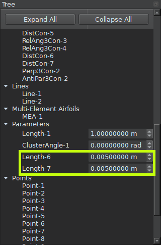
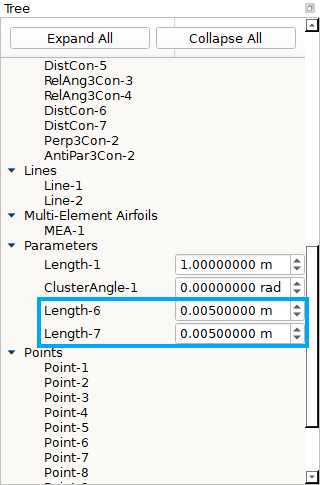
Next, we see from inspection that the NACA 0012 has its trailing edge upper surface point located at \((1.0,0.00126)\) and its trailing edge lower surface point at \((1.0,-0.00126)\). To set the trailing edge thickness accordingly, we need to set the values of "Length-6" and "Length-7", which control the distances between the \((1,0)\) point and the trailing edge upper surface point and trailing edge lower point, respectively. To do this, either double-click on the trailing edge thickness lengths in the canvas, change each value to 0.00126, and left-click elsewhere on the canvas, or simply type in this number in the parameter tree in the spin boxes for both "Length-7".

Modifying trailing edge thickness

Modifying trailing edge thickness

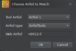
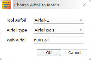
The airfoil is now ready to be matched. To match the airfoil, open the airfoil-matching dialog using Tools → Match Airfoil. Make sure that Airfoil-1 is selected as the tool airfoil, the “Airfoil Type” is set to AirfoilTools, and the “Web Airfoil” is set to n0012-il. Then, press “OK.”

Airfoil matching dialog

Airfoil matching dialog

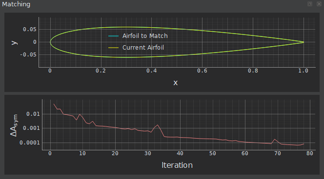
A new tab should appear that shows the morphing of the airfoil shape during the optimization and a graph of the objective function value. In this case, the optimizer gives a final objective function value of \(\Delta A_\text{sym}=1.211 \times 10^{-4}\). Save the updated airfoil using File → Save As.

Airfoil matching graph

Airfoil matching graph

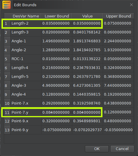
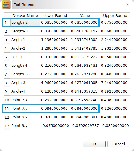
This is a good match for an airfoil with a chord length of 1. We can potentially achieve a better match by expanding the variable bounds and adding control points. We can pull up the design variables bounds editor using Edit → Bounds or by pressing Ctrl+B. Notice that both design variable 1 (Length-2) and design variable 11 (Point-7.x) have values equal to their lower bounds, which means that expanding the bounds could potentially allow the optimizer to achieve a better match. Modify the lower bounds by double-clicking and replacing the lower bounds of Length-2 and Point-7.x with 0.02 and 0.2, respectively.

Editing variable bounds

Editing variable bounds

Matching the airfoil again with these modified lower bounds gives a slightly higher objective function value than before, which indicates that the optimization might be getting stuck in a local minimum. However, tuning these bounds and the bounds of other design variables can possibly drive the objective function value further down.

Another strategy to get a closer match is the addition of curve control points. First, load in the previously saved .jmea file from the first matching using File → Open. We can add one control point to each of the airfoil surfaces by left-clicking inside the airfoil canvas, pressing p (or by clicking on the Point button in the tool bar), and placing points somewhere near \((0.6,0.08)\) and \((0.6,-0.08)\). Double-click on the newly created point references in the Parameter Tree to set the \(x\)- and \(y\)-values equal to these numbers if desired. Next, add the points to their respective curves by left-clicking the curve, then right-clicking and selecting Modify Geometry → Insert Curve Point and following the instructions that appear in the status bar (lower left-hand corner of the GUI).

Airfoil matching graph after adding two control points

Airfoil matching graph after adding two control points

To add the \(x\)- and \(y\)-locations of these points as design variables, right-click on their references in the parameter tree and select “Expose x and y Parameters” from the context menu. Then, select the newly created parameters (Point-13.x, Point-13.y, Point-14.x, and Point-14.y), right-click on their references, and select “Promote to Design Variable” from the context menu. Matching this airfoil with four additional design variables gives an improved objective function value of \(\Delta A_\text{sym}=8.371 \times 10^{-5}\), an excellent match. Do not forget to save the matched airfoil if necessary!

API

To get a parametrization to start with, we load in the “Single Airfoil (Blunt TE)” example from pymead’s example directory:

from pymead.core.geometry_collection import GeometryCollection

geo_col = GeometryCollection.load_example("basic_airfoil_blunt_dv")

Next, we see from inspection that the NACA 0012 has its trailing edge upper surface point located at \((1.0,0.00126)\) and its trailing edge lower surface point at \((1.0,-0.00126)\). To set the trailing edge thickness accordingly, we need to set the values of "Length-6" and "Length-7", which control the distances between the \((1,0)\) point and the trailing edge upper surface point and trailing edge lower point, respectively:

geo_col.container()["params"]["Length-6"].set_value(0.00126)
geo_col.container()["params"]["Length-7"].set_value(0.00126)

Now, we can match the airfoil and update the GeometryCollection with the result:

from pymead.optimization.airfoil_matching import match_airfoil
opt_result = match_airfoil(None, geo_col.get_dict_rep(), "Airfoil-1", "n0012-il")
geo_col.assign_design_variable_values(opt_result.x, bounds_normalized=True)

The optimizer gives a final objective function value of \(\Delta A_\text{sym}=1.211 \times 10^{-4}\), which is a good match for an airfoil with a chord length of 1. We can potentially achieve a better match by expanding the variable bounds and adding control points. Inspecting the resulting list of bounds-normalized design variable values, given by opt_result.x, we see that the variables at index 0 and index 10 both have a value of 0.0, which means that those design variables are exactly at their lower bounds. We can see the dimensional value of these variables using the following code:

dv_key_list = list(geo_col.container()["desvar"].keys())
dv_0 = geo_col.container()["desvar"][dv_key_list[0]]
dv_10 = geo_col.container()["desvar"][dv_key_list[10]]
print(f"Design variable 0 ({dv_0.name()}) has lower bound {dv_0.lower()} and value {dv_0.value()}")
print(f"Design variable 10 ({dv_10.name()}) has lower bound {dv_10.lower()} and value {dv_10.value()}")

We can update the value of these lower bounds to lower values:

dv_0.set_lower(0.02)
dv_10.set_lower(0.2)

Running the matching function again gives a result with a slightly higher objective function value, which indicates that the optimization might be getting stuck in a local minimum. However, tuning these bounds and the bounds of other design variables can possibly drive the objective function value further down. Another strategy to get a closer match is the addition of curve control points. We can add one control point to each of the airfoil surfaces:

new_upper_point = geo_col.add_point(0.6, 0.08)
new_lower_point = geo_col.add_point(0.6, -0.08)
upper_bezier = geo_col.container()["bezier"]["Bezier-1"]
lower_bezier = geo_col.container()["bezier"]["Bezier-2"]
upper_bezier.point_sequence().insert_point(4, new_upper_point)
lower_bezier.point_sequence().insert_point(4, new_lower_point)

To add the \(x\)- and \(y\)-locations of these points as design variables, we can use the following code:

geo_col.expose_point_xy(new_upper_point)
geo_col.expose_point_xy(new_lower_point)
for xy_param in [new_upper_point.x(), new_upper_point.y(), new_lower_point.x(), new_lower_point.y()]:
    geo_col.promote_param_to_desvar(xy_param)

The GeometryCollection.promote_param_to_desvar also allows the specifications of lower and upper bounds to be added on promotion. Leaving these values as None (not specifying them) allows pymead to choose reasonable lower and upper bounds to start with. Matching this airfoil with the additional control points added (note that we started from the result of the very first optimization with the original bounds on the design variables at index 0 and index 10), we get a better match with \(\Delta A_\text{sym}=8.371 \times 10^{-5}\).