Continuity#

There are different kinds of continuity frequently discussed in computer graphics design: geometric continuity (or \(G^k\) continuity) and parametric continuity (or \(C^k\) continuity). Geometric continuity requires that two joined curves have continuity in the geometry at the curve junction. Parametric continuity is stricter in that it also requires that the parameter describing the curve is also continuous across the curve junction. This is done by requiring that the \(k\)-th order derivative is equal at the junction.

Because parametric continuity is stricter than geometric continuity, it also limits a degree of freedom at the curve junction, which may or may not be desirable from an airfoil design perspective. In addition, \(G^2\) continuity requires an equal radius of curvature of both curves at the curve junction. This allows for direct control over the radius of curvature at each curve junction, which is a nice feature from an airfoil design standpoint. It is for both of these reasons that pymead chooses to enforce geometric, rather than parametric, continuity across each curve junction. In particular, \(G^0\) (point) continuity, \(G^1\) (slope) continuity, and \(G^2\) (curvature) continuity are enforced at the joint between each set of Bézier curves in the airfoil.

Note

One drawback of using geometric, rather than parametric, continuity is that in some cases, the distance traveled by the curve with an equal change in parameter value can change significantly across a curve joint. However, for practical purposes, as long as a sufficiently small change in parameter (\(\Delta t \lessapprox 0.01\)) is chosen, there will be little difference either from a graphical or aerodynamic perspective. If this does make a difference aerodynamically (e.g., if the airfoil is being used in a panel code), the parameter vector density can be increased, or the parameter vector can take non-linear spacing (e.g., cosine spacing or curvature-based spacing).

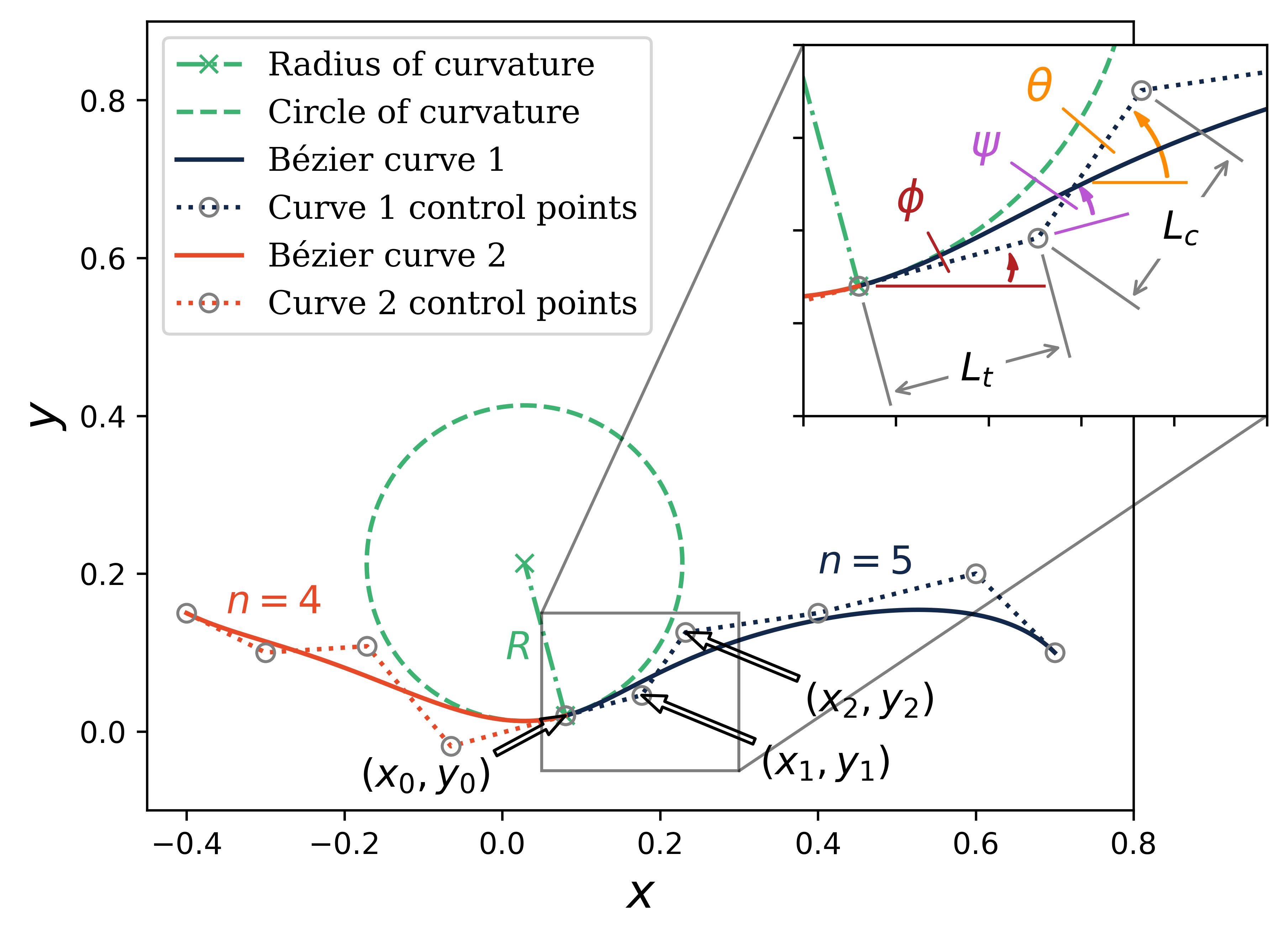
The enforcement of point continuity is straightforward; the end control point location of one Bézier curve just needs to match the start control point location of the next Bézier curve. Slope continuity is similarly straightforward. The slope of the line connecting the second-to-last and last control points of one Bézier curve must match the slope of the line connecting the first and second control points of the next Bézier curve. Curvature continuity, on the other hand, is not so straightfoward to enforce. In pymead, curvature continuity is enforced by specifying a radius of curvature and an angle of the second-to-last control point segment relative to the first control point segment. Then, the length of this second-to-last control point segment is chosen according to the following equation:

\[L_c = \frac{L_t^2}{R\left(1 - \frac{1}{n} \right) \sin{\psi}}\]

Here, \(L_c\) is the length of the curvature control arm (second-to-last control point segment), \(L_t\) is the length of the slope control arm (last control point segment), \(R\) is the radius of curvature at the curve joint, \(n\) is the Bézier curve order, and \(\psi\) is the angle of the curvature control arm relative to the slope control arm. A geometric description of \(\psi\) is shown below:

../_images/bezier_g2_diagram_dark.png — Bézier G² continuity#

../_images/bezier_g2_diagram_light.png — Bézier G² continuity#

A derivation of the above equation is reserved for a journal paper (coming soon).